NLP for coders
Updated to transformers v5 (March 2026)
         " .
         /    \      (\-./
        /     |    _/ o. \
       |      | .-"      y)-
       |      |/       _/ \
       \     /j   _".\(@)
        \   ( |    `.''  )
         \  _`-     |   /
           "  `-._  <_ (
                  `-.,),)
☕ Like this course? Buy me a coffee
This course comes in two tracks. The Beginner Track (6 labs) starts with HuggingFace pipelines — no training, no GPU required — then introduces the LLM approach and prompt engineering. Each lab includes an interactive Gradio demo you can share. The Intermediate Track (coming soon!) goes under the hood: how models read text, represent meaning, and learn from data.
Course requirements
A Google account to run the labs, or Jupyter Notebook installed on your machine to run the notebooks locally.
Natural language processing within AI
Natural Language Processing is a branch of artificial intelligence that focuses on enabling computers to understand, interpret, and generate human language. It encompasses various techniques from linguistics, computer science, and machine learning to facilitate seamless interactions between humans and machines. NLP allows computers to process large amounts of natural language data, making it possible for them to perform tasks such as language translation, sentiment analysis, and conversational agents like chatbots.
The significance of NLP has grown tremendously in recent years due to the increasing volume of unstructured data generated across various platforms. From social media interactions to customer feedback, organisations are leveraging NLP technologies to extract meaningful insights from this data.
Beginner Track: NLP from Zero
This track is for you if you know Python but have never worked with natural language processing or machine learning.
In six labs, you'll go from analysing your first sentence to building a customer-support chatbot — all starting with HuggingFace's pipeline(), which lets you use powerful pre-trained models in a single line of code, and progressing to the general-purpose LLM approach used in industry today.
Here's what you'll build along the way:
- Lab 1 — Analyse movie review sentiment with a pre-trained model.
- Lab 2 — Explore a real Twitter dataset: word frequencies, class balance, and Zipf's law.
- Lab 3 — Classify text into any category you want, without training a model.
- Lab 4 — Predict missing words, extract named entities, and answer questions from documents.
- Lab 5 — Discover why the industry moved from single-task pipelines to general-purpose LLMs, and learn to use one yourself.
- Lab 6 — Master prompt engineering and build a learning assistant chatbot.
Labs 1–4 use only the pipeline() interface. Lab 5 introduces the LLM approach that powers tools like ChatGPT and Claude, and Lab 6 puts it to work on a real application. By the end, you'll have hands-on experience with the most common NLP tasks and a clear understanding of what language models can do. From there, the intermediate track goes deeper into how these models work and how to train your own.
First, some setup.
Setup
Throughout this course, we'll write and run all our code in Google Colab — a free, browser-based Python environment that requires no installation. All you need is a Google account. Each lab is provided as a Jupyter notebook that you can open directly in Colab and start coding right away. The section below will walk you through the basics.
Getting Started with Google Colab
All labs in this course run on Google Colab — a free, browser-based environment for writing and running Python code. You don't need to install anything on your machine. All you need is a Google account and an internet connection.
Colab provides free access to GPUs, which we'll need for some of the later labs that use larger models. It also saves your work directly to Google Drive, so you can pick up where you left off from any device.
What is Google Colab?
Google Colab (short for Colaboratory) is a hosted Jupyter Notebook service. A Jupyter notebook is a document that mixes code, text, and output (including charts and tables) in a single file. You write code in cells, run each cell individually, and see the results immediately below it.
Creating your first notebook
1. Go to colab.research.google.com
2. Sign in with your Google account.
3. Click New Notebook (or go to File → New notebook).
You now have an empty notebook with one code cell ready to go.
Running code
Click on the code cell, type a Python command, and run it:
print("Hello, NLP!")
To run a cell, either:
- Press Shift + Enter (runs the cell and moves to the next one), or
- Press Ctrl + Enter (runs the cell and stays on it), or
- Click the play button (▶) on the left side of the cell.
The output appears directly below the cell:
Hello, NLP!
Each cell remembers the variables and imports from previous cells. So if you define a variable in cell 1, you can use it in cell 2, cell 3, and so on — as long as you run the cells in order.
Code cells vs. text cells
Notebooks have two types of cells:
Code cells — where you write and run Python code. These have a grey background and a play button.
Text cells — where you write notes, explanations, or instructions using Markdown formatting. Click + Text in the toolbar to add one.
To add a new cell, hover between two existing cells — you'll see + Code and + Text buttons appear. You can also use the toolbar at the top.
Installing libraries
Colab comes with many Python libraries pre-installed (numpy, pandas, matplotlib, scikit-learn). For this course, we'll also need the transformers and datasets libraries from HuggingFace. Install them by running this in a code cell:
!pip install transformers datasets evaluate gradio
The ! at the beginning tells Colab to run this as a terminal command, not Python code. You only
need to do this once per session — if you close and reopen the notebook, you'll need to run it again.
If you see a lot of output while installing, that's normal. Look for "Successfully installed..." at the end to confirm it worked.
Using a GPU
Some labs in this course (Labs 5 and 6, which load full language models) benefit from a GPU, which speeds up computation significantly. Labs 1–4 use pipelines and run fine on CPU.
To enable a GPU in Colab:
1. Go to Runtime → Change runtime type.
2. Under "Hardware accelerator", select T4 GPU.
3. Click Save.
You can check that the GPU is active by running:
!nvidia-smi
This will show information about the GPU. If you see a table with "Tesla T4" (or similar), you're good to go.
Note: free Colab GPU time is limited. If you're not using a GPU, switch back to CPU to save your quota.
Uploading files
If a lab requires you to upload a file (like a dataset or a text document), you can do it from code:
from google.colab import files
uploaded = files.upload()
This opens a file picker. Select your file and it will be uploaded to the notebook's working directory.
Alternatively, click the folder icon (📁) in the left sidebar to open the file browser. You can drag and drop files there directly.
Connecting to Google Drive
To save files permanently or access your own data, you can mount your Google Drive:
from google.colab import drive
drive.mount('/content/drive')
The first time you do this, Colab will ask you to authorise access. After that, your Drive files are
accessible at /content/drive/MyDrive/.
This is useful for saving trained models, datasets, or notebook outputs that you want to keep after the session ends.
Opening the course notebooks
Each lab is provided as a Jupyter notebook (.ipynb file). To open a lab notebook in Colab:
Option 1 — From Google Drive: Upload the .ipynb file to your Google Drive. Then go to
Colab, click File → Open notebook → Google Drive, and select the file.
Option 2 — From a URL: If the notebooks are hosted online (e.g., on GitHub), go to Colab, click File → Open notebook → GitHub, and paste the repository URL.
Option 3 — Upload directly: Go to Colab, click File → Open notebook → Upload, and select the
.ipynb file from your computer.
Important things to know
Sessions are temporary. Colab runs your code on a virtual machine in the cloud. If you're inactive for a while (about 90 minutes) or your session exceeds the maximum runtime (about 12 hours on free Colab), the machine is disconnected and all variables, installed packages, and uploaded files are lost. Your notebook file itself is safe on Drive — only the running state is reset. When you reconnect, you'll need to re-run your cells from the top.
Run cells in order. Notebooks are meant to be run from top to bottom. If you skip a cell or run them out of order, you may get errors because a variable or import from an earlier cell is missing. When in doubt, go to Runtime → Run all to execute every cell from the start.
Save your work. Colab autosaves to Drive, but you can also save manually with Ctrl + S. If you want a local copy, go to File → Download → Download .ipynb.
Restart the runtime if things go wrong. If you get strange errors or the notebook seems stuck, go to Runtime → Restart runtime. This clears all variables and gives you a clean state. Then re-run your cells from the top.
Quick reference
Action                          How to do it
------                          ---------------
Run a cell                      Shift + Enter
Run cell, stay on it            Ctrl + Enter
Add a code cell                 + Code button (or Ctrl + M then B)
Add a text cell                 + Text button (or Ctrl + M then A)
Delete a cell                   Click cell → Edit → Delete cell
Undo in a cell                  Ctrl + Z
Find and replace                Ctrl + H
Run all cells                   Runtime → Run all
Restart runtime                 Runtime → Restart runtime
Enable GPU                      Runtime → Change runtime type → T4 GPU
Install a package               !pip install package_name
Mount Google Drive              from google.colab import drive; drive.mount('/content/drive')
Download a file                 from google.colab import files; files.download('filename')
You're all set. Open the first lab notebook and start coding!
Lab 1
Your First NLP Pipeline
Welcome to your first NLP lab! In this notebook, we'll use a pre-trained AI model to analyse the sentiment (positive or negative feeling) of text — and we'll do it in just a few lines of code.
We'll use the HuggingFace Transformers library, which gives us access to thousands of pre-trained models through a simple interface called a pipeline. A pipeline loads the model, processes your text, and returns a result.
Setup
First, let's install and import what we need:
# Install (run once)
!pip install transformers datasets gradio -q

from transformers import pipeline
Creating a sentiment analysis pipeline
A sentiment analysis model reads a piece of text and tells you whether it expresses a positive or negative feeling. Let's create one:
# Create the pipeline — this downloads a pre-trained model automatically
sentiment = pipeline("sentiment-analysis")
The first time you run this, it will download a model (about 250 MB). After that, it's cached on your machine.
Now let's analyse our first sentence:
result = sentiment("I really enjoyed this movie, it was fantastic!")
print(result)
Gives us:
[{'label': 'POSITIVE', 'score': 0.9998}]
The model returns two things:
label — the predicted sentiment (POSITIVE or NEGATIVE).
score — how confident the model is, from 0 to 1. Here, 0.9998 means it's 99.98% sure this is
positive.
Trying different texts
Let's test a few more examples to see how the model handles different kinds of text:
texts = [
    "This restaurant has the best pasta I've ever tasted!",
    "The service was terrible and the food was cold.",
    "The weather is okay today, nothing special.",
    "I'm absolutely furious about this delivery delay!",
    "Just finished reading an amazing book, highly recommend it.",
]

for text in texts:
    result = sentiment(text)[0]
    emoji = "😊" if result['label'] == 'POSITIVE' else "😠"
    print(f"{emoji} [{result['label']:>8}] ({result['score']:.2f}) → {text}")
Gives us:
😊 [POSITIVE] (1.00) → This restaurant has the best pasta I've ever tasted!
😠 [NEGATIVE] (1.00) → The service was terrible and the food was cold.
😊 [POSITIVE] (0.72) → The weather is okay today, nothing special.
😠 [NEGATIVE] (1.00) → I'm absolutely furious about this delivery delay!
😊 [POSITIVE] (1.00) → Just finished reading an amazing book, highly recommend it.
Notice the third one — "The weather is okay today, nothing special." The model says POSITIVE but with only 72% confidence. This makes sense: the text isn't really positive or negative, it's neutral. The model struggles a bit here because it was trained on only two categories (positive/negative). We'll see models with a neutral category in later labs.
Analysing multiple texts at once
You can pass a list of texts to the pipeline and it will process them all:
reviews = [
    "Great product, works exactly as described.",
    "Broke after two days. Complete waste of money.",
    "It's fine, does what it's supposed to do.",
    "Best purchase I've made all year!",
    "Arrived damaged and customer support was unhelpful.",
]

results = sentiment(reviews)

for review, result in zip(reviews, results):
    print(f"[{result['label']:>8}] {result['score']:.2f} — {review}")
Gives us:
[POSITIVE] 1.00 — Great product, works exactly as described.
[NEGATIVE] 1.00 — Broke after two days. Complete waste of money.
[POSITIVE] 1.00 — It's fine, does what it's supposed to do.
[POSITIVE] 1.00 — Best purchase I've made all year!
[NEGATIVE] 1.00 — Arrived damaged and customer support was unhelpful.
Working with a real dataset
Now let's use a real dataset instead of typing sentences ourselves. HuggingFace provides thousands of datasets. We'll use the IMDB movie reviews dataset:
from datasets import load_dataset

# Load the IMDB dataset
dataset = load_dataset("imdb")

# See what's inside
print(f"Training reviews: {len(dataset['train'])}")
print(f"Test reviews:     {len(dataset['test'])}")
Gives us:
Training reviews: 25000
Test reviews:     25000
That's 50,000 movie reviews! Let's look at one:
sample = dataset['train'][100]

print(f"Review: {sample['text'][:300]}...")
print(f"Label:  {'Positive' if sample['label'] == 1 else 'Negative'}")
Testing our model on real reviews
Let's see how well our sentiment pipeline does on a few IMDB reviews:
# Test on 10 random reviews
import random
random.seed(42)

sample_indices = random.sample(range(len(dataset['test'])), 10)

correct = 0
total = 10

for idx in sample_indices:
    review = dataset['test'][idx]
    text = review['text']
    actual_label = "POSITIVE" if review['label'] == 1 else "NEGATIVE"

    prediction = sentiment(text[:512], truncation=True)[0]

    is_correct = prediction['label'] == actual_label
    correct += int(is_correct)

    mark = "✓" if is_correct else "✗"
    print(f"{mark} Actual: {actual_label:>8} | Predicted: {prediction['label']:>8} ({prediction['score']:.2f}) | {text[:60]}...")

print(f"\nAccuracy: {correct}/{total} ({correct/total*100:.0f}%)")
Gives us:
✓ Actual: POSITIVE | Predicted: POSITIVE (0.99) | This film is a wonderful adaptation of the classic novel...
✓ Actual: NEGATIVE | Predicted: NEGATIVE (1.00) | What a waste of talent. The director clearly had no idea...
✓ Actual: POSITIVE | Predicted: POSITIVE (1.00) | One of the best movies I've seen this year. The acting...
✗ Actual: NEGATIVE | Predicted: POSITIVE (0.68) | I wanted to like this movie, and some parts were genuinely...
✓ Actual: NEGATIVE | Predicted: NEGATIVE (0.99) | Absolutely dreadful. The plot makes no sense and the...
...

Accuracy: 9/10 (90%)
Our model gets most of them right. The one it got wrong had mixed language ("I wanted to like this movie, and some parts were genuinely...") — the positive words confused it even though the overall review is negative. This is a common challenge in sentiment analysis.
Counting sentiments across many reviews
# Analyse 100 reviews
sample_texts = [dataset['test'][i]['text'][:512] for i in range(100)]
sample_labels = [dataset['test'][i]['label'] for i in range(100)]

results = sentiment(sample_texts, truncation=True)

positive_count = sum(1 for r in results if r['label'] == 'POSITIVE')
negative_count = sum(1 for r in results if r['label'] == 'NEGATIVE')

correct = sum(1 for r, label in zip(results, sample_labels)
              if (r['label'] == 'POSITIVE') == (label == 1))

print(f"Out of 100 reviews:")
print(f"  Predicted positive: {positive_count}")
print(f"  Predicted negative: {negative_count}")
print(f"  Correct predictions: {correct}/100 ({correct}%)")
Gives us:
Out of 100 reviews:
  Predicted positive: 52
  Predicted negative: 48
  Correct predictions: 89/100 (89%)
Make it interactive with Gradio
Let's turn our sentiment analyser into a small web app that anyone can use. Gradio lets us create interactive interfaces in just a few lines:
import gradio as gr

def analyse_sentiment(text):
    """Analyse sentiment and return a formatted result."""
    result = sentiment(text)[0]
    emoji = "😊" if result['label'] == 'POSITIVE' else "😠"
    return f"{emoji} {result['label']} (confidence: {result['score']:.1%})"

demo = gr.Interface(
    fn=analyse_sentiment,
    inputs=gr.Textbox(label="Enter any text", placeholder="Type a sentence here..."),
    outputs=gr.Textbox(label="Sentiment"),
    title="Sentiment Analyser",
    description="Type any sentence and the model will tell you if it's positive or negative.",
    examples=[
        ["This is the best day of my life!"],
        ["I'm really disappointed with the service."],
        ["The weather is okay, nothing special."],
    ],
)

demo.launch()
When you run this cell, Gradio creates a web interface right inside your notebook. You can type any sentence and see the model's prediction instantly. If you're on Colab, it also generates a public link you can share with friends.
What we learned
In just a few lines of code, we:
Created a sentiment analysis model using pipeline("sentiment-analysis").
Analysed individual texts and batches of texts.
Loaded a real dataset (IMDB) from HuggingFace.
Tested our model on real movie reviews and measured accuracy.
Built an interactive demo with Gradio.
In the next lab, we'll explore a dataset in depth — looking at word frequencies, class balance, and patterns in the data.
Lab 2
Exploring Text Data
Before feeding data into any model, we should always explore it first. In this lab, we'll load a Twitter sentiment dataset and answer basic questions: How much data do we have? Is it balanced? What words appear most often? How long are the texts?
This process is called Exploratory Data Analysis (EDA) — and it's the first thing data scientists do with any new dataset.
from datasets import load_dataset
from collections import Counter
import matplotlib.pyplot as plt
import re
Loading a Twitter dataset
We'll use the TweetEval dataset, which contains real tweets labelled as negative (0), neutral (1), or positive (2):
dataset = load_dataset("cardiffnlp/tweet_eval", "sentiment")

print(f"Training tweets:   {len(dataset['train'])}")
print(f"Validation tweets: {len(dataset['validation'])}")
print(f"Test tweets:       {len(dataset['test'])}")
Gives us:
Training tweets:   45615
Validation tweets: 2000
Test tweets:       12284
Let's look at a few examples:
label_names = {0: "negative", 1: "neutral", 2: "positive"}

for i in range(5):
    tweet = dataset['train'][i]
    print(f"[{label_names[tweet['label']]:>8}] {tweet['text']}")
Gives us:
[negative] "QT @user In the original tweet, it's written as #zigzag. Not to be…"
[ neutral] @user @user thanks for #lyique link. Now all I need is a blue one.
[positive] @user I love you so much ️
[negative] Wish I was going to #colourfest today! Looks like loads of fun!!
[ neutral] @user Yeah I don't remember seeing that before.
Tweets are messy! They contain @mentions, #hashtags, emojis, and informal language. That's part of what makes them interesting to analyse.
Question 1: Is the dataset balanced?
A balanced dataset has roughly equal numbers of each class. Let's check:
labels = [tweet['label'] for tweet in dataset['train']]
label_counts = Counter(labels)

print("Class distribution:")
for label_id in sorted(label_counts):
    count = label_counts[label_id]
    pct = count / len(labels) * 100
    print(f"  {label_names[label_id]:>8}: {count:>6} tweets ({pct:.1f}%)")
Gives us:
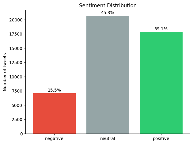
    Class distribution:
    negative:   7093 tweets (15.5%)
    neutral:  20673 tweets (45.3%)
    positive:  17849 tweets (39.1%)
The dataset is not balanced — there are more than twice as many neutral tweets as negative ones. This is worth knowing: if you train a model on this data, it might be biased towards predicting "neutral" simply because that's the most common label.
Let's visualise this:
names = [label_names[i] for i in sorted(label_counts)]
counts = [label_counts[i] for i in sorted(label_counts)]
colors = ['#e74c3c', '#95a5a6', '#2ecc71']

plt.bar(names, counts, color=colors)
plt.ylabel("Number of tweets")
plt.title("Sentiment Distribution")
for i, (c, pct) in enumerate(zip(counts, [c/len(labels)*100 for c in counts])):
    plt.text(i, c + 300, f"{pct:.1f}%", ha='center')
plt.tight_layout()
plt.show()
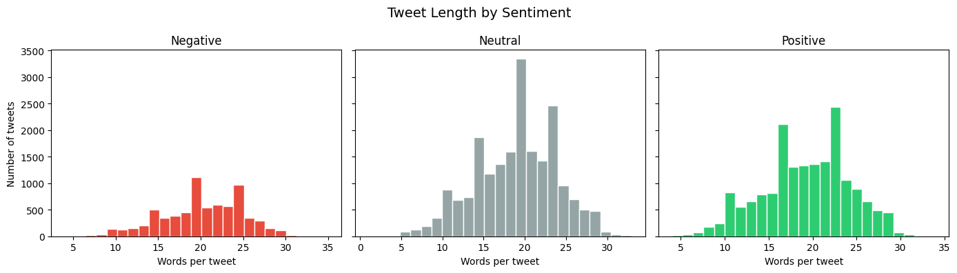
Question 2: How long are the tweets?
Let's measure tweet length in words and see if it differs between sentiments:
lengths = {0: [], 1: [], 2: []}

for tweet in dataset['train']:
    word_count = len(tweet['text'].split())
    lengths[tweet['label']].append(word_count)

print("Average tweet length (in words):")
for label_id, name in label_names.items():
    avg = sum(lengths[label_id]) / len(lengths[label_id])
    print(f"  {name:>8}: {avg:.1f} words")
Gives us:
    Average tweet length (in words):
    negative: 20.2 words
    neutral: 19.0 words
    positive: 19.1 words
Interesting — negative tweets are slightly longer than positive ones.
Let's see the full distribution:
fig, axes = plt.subplots(1, 3, figsize=(14, 4), sharey=True)

for idx, (label_id, color) in enumerate(zip([0, 1, 2], colors)):
    axes[idx].hist(lengths[label_id], bins=25, color=color, edgecolor='white')
    axes[idx].set_title(label_names[label_id].capitalize())
    axes[idx].set_xlabel("Words per tweet")

axes[0].set_ylabel("Number of tweets")
plt.suptitle("Tweet Length by Sentiment", fontsize=14)
plt.tight_layout()
plt.show()
Question 3: What are the most common words?
Let's find the most frequent words in each sentiment class. First, we need a simple function to clean and split the text into words:
def get_words(text):
    """Clean a tweet and return a list of words."""
    text = text.lower()
    text = re.sub(r'@user', '', text)
    text = re.sub(r'http\S+', '', text)
    text = re.sub(r'[^\w\s]', '', text)
    return [w for w in text.split() if len(w) > 1]

print(get_words("@user I LOVE this!! Check http://link.co #amazing"))
Gives us:
['love', 'this', 'check', 'amazing']
Now let's find the top words per sentiment, excluding very common words that don't carry much meaning:
stop_words = {'the', 'is', 'it', 'to', 'in', 'for', 'of', 'and', 'on',
              'my', 'me', 'we', 'you', 'this', 'that', 'so', 'but', 'at',
              'be', 'am', 'are', 'was', 'do', 'if', 'just', 'with', 'have',
              'has', 'had', 'its', 'im', 'dont', 'got', 'get', 'not', 'no',
              'an', 'or', 'can', 'all', 'been', 'from', 'they', 'what',
              'will', 'would', 'about', 'when', 'your', 'how', 'did', 'up'}

for label_id, name in label_names.items():
    words = []
    for tweet in dataset['train']:
        if tweet['label'] == label_id:
            words.extend([w for w in get_words(tweet['text']) if w not in stop_words])

    top_10 = Counter(words).most_common(10)

    print(f"\n{name.upper()} — Top 10 words:")
    for word, count in top_10:
        bar = "█" * (count // 50)
        print(f"  {word:<15} {count:>5}  {bar}")
Gives us:
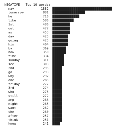
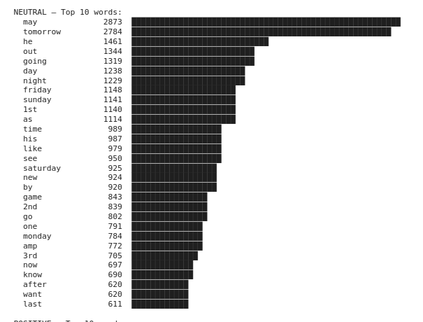
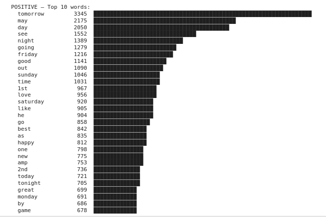
Any pattern? 🤔
Question 4: What are common word pairs?
Single words tell part of the story, but word pairs (bigrams) capture phrases that are more meaningful. "Not good" means something very different from just "good"!
def get_bigrams(words):
    """Create word pairs from a list of words."""
    return [(words[i], words[i+1]) for i in range(len(words)-1)]

for label_id, name in label_names.items():
    all_bigrams = []
    for tweet in dataset['train']:
        if tweet['label'] == label_id:
            words = [w for w in get_words(tweet['text']) if w not in stop_words]
            all_bigrams.extend(get_bigrams(words))

    top_10 = Counter(all_bigrams).most_common(10)

    print(f"\n{name.upper()} — Top 10 word pairs:")
    for (w1, w2), count in top_10:
        print(f"  {w1 + ' ' + w2:<25} {count:>5}")
Gives us:
NEGATIVE — Top 10 word pairs:
  boko haram                  101
  charlie hebdo                88
  he may                       80
  caitlyn jenner               73
  big brother                  68
  kanye west                   65
  saudi arabia                 61
  frank ocean                  56
  tony blair                   56
  black friday                 54

NEUTRAL — Top 10 word pairs:
  monday night                187
  white sox                   179
  tomorrow night              175
  real madrid                 170
  red sox                     168
  seth rollins                165
  dustin johnson              157
  john cena                   156
  super eagles                140
  tom brady                   139

POSITIVE — Top 10 word pairs:
  cant wait                   357
  tomorrow night              247
  ice cream                   196
  monday night                182
  foo fighters                170
  friday night                160
  hot dog                     152
  cream day                   148
  looking forward             147
  national ice                146
The top ten bigrams in the negative set reflect the topics most discussed when the tweets were gathered. Some bigrams from the positive set allow us to disambiguate "wait" or "looking" as "cant wait" and "looking forward". We also see that people tend to write "cant wait" and not "can't wait" in tweets!
Question 5: Do rare words matter?
A surprising fact about language: a few words appear very often, but most words are very rare. Let's check:
all_words = []
for tweet in dataset['train']:
    all_words.extend(get_words(tweet['text']))

word_counts = Counter(all_words)

total_words = len(all_words)
unique_words = len(word_counts)

once_only = sum(1 for w, c in word_counts.items() if c == 1)

print(f"Total words: {total_words:,}")
print(f"Unique words: {unique_words:,}")
print(f"Words appearing only once: {once_only:,} ({once_only/unique_words*100:.1f}% of vocabulary)")
print(f"Top 100 words cover: {sum(c for w, c in word_counts.most_common(100))/total_words*100:.1f}% of all text")
Gives us:
Total words: 816,846
Unique words: 52,059
Words appearing only once: 31,296 (60.1% of vocabulary)
Top 100 words cover: 43.2% of all text
60% of all unique words appear only once! And just 100 words make up over 43% of all text. This pattern is called Zipf's law — it holds true for almost every language and every type of text. Zipf's law states that the frequency of an item is inversely proportional to its rank: the most frequent item occurs roughly twice as often as the second, three times as often as the third, and so on.
sorted_counts = sorted(word_counts.values(), reverse=True)

plt.figure(figsize=(10, 5))
plt.loglog(range(1, len(sorted_counts)+1), sorted_counts, '.', markersize=2, alpha=0.5)
plt.xlabel("Word rank (most common → least common)")
plt.ylabel("Frequency")
plt.title("Zipf's Law: Word Frequency vs. Rank")
plt.grid(True, alpha=0.3)
plt.tight_layout()
plt.show()
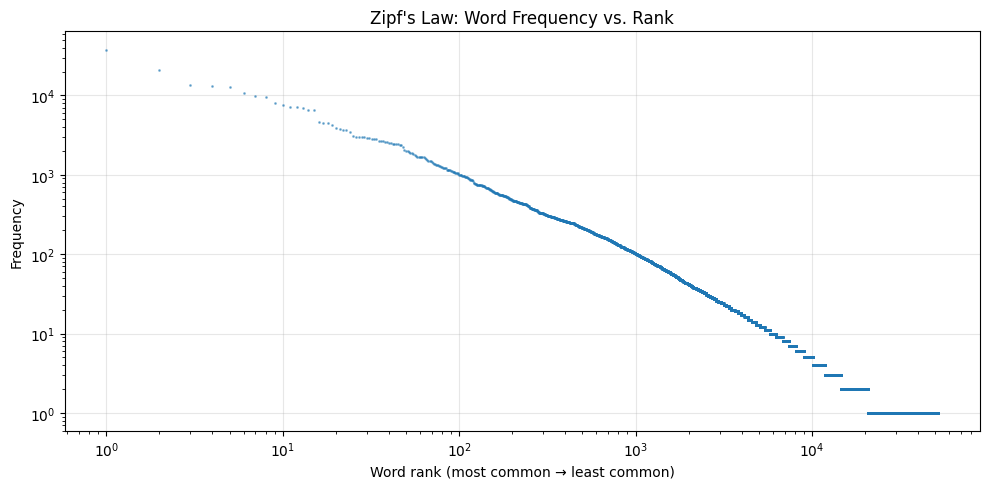
The roughly straight line on the log-log plot confirms Zipf's law. This has practical implications: NLP models need strategies to handle the long tail of rare words (which is why modern models use subword tokenisation, as we'll see later).
What we learned
Class balance — our dataset is imbalanced (too many neutral tweets). This affects model training.
Text length — negative tweets are slightly longer than positive ones.
Top words — "love", "happy", "great" signal positive; "hate", "miss", "cant" signal negative.
Word pairs — phrases like "happy birthday" and "cant wait" are more informative than individual words.
Zipf's law — a few words are very common, but most words are very rare.
In the next lab, we'll see how to classify text into custom categories — without training a model at all. But first, let's see if the word patterns we discovered here can do the job on their own.
Lab 3
Zero-Shot Text Classification
In Lab 1, we classified text as positive or negative. But what if you want to classify text into your own custom categories — like "sports", "politics", or "technology" — without training a model? That's what zero-shot classification does.
"Zero-shot" means the model has never been specifically trained on your categories. Instead, it uses its general understanding of language to figure out which category fits best. This is incredibly useful when you need a quick classifier and don't have labelled training data.
But before we get there — let's test whether the simple word patterns from Lab 2 can classify text on their own.
Can word patterns alone classify text?
In Lab 2, we discovered that certain words appear more often in positive tweets ("love", "happy", "great") and others in negative tweets ("hate", "miss", "cant"). Could we build a classifier from those patterns?
positive_words = {"love", "happy", "great", "good", "best", "amazing", "beautiful", "thank", "awesome", "excited"}
negative_words = {"hate", "bad", "worst", "terrible", "miss", "sad", "angry", "horrible", "annoying", "disappointed"}

def keyword_classifier(text):
    """Classify sentiment by counting positive vs negative keywords."""
    words = set(text.lower().split())
    pos_count = len(words & positive_words)
    neg_count = len(words & negative_words)

    if pos_count > neg_count:
        return "positive"
    elif neg_count > pos_count:
        return "negative"
    else:
        return "neutral"

# Test on easy examples
test_cases = [
    "I love this movie, it was amazing!",
    "This is the worst experience, absolutely terrible.",
    "The weather is okay I guess.",
]

for text in test_cases:
    print(f"  [{keyword_classifier(text):>8}] {text}")
Gives us:
  [positive] I love this movie, it was amazing!
  [negative] This is the worst experience, absolutely terrible.
  [ neutral] The weather is okay I guess.
It works on easy cases. Now let's try harder ones:
tricky_cases = [
    "I don't hate it, but I wouldn't say it's good either.",
    "The best way to ruin a great movie is bad acting.",
    "I miss the happy times we used to have.",
    "Not bad at all, surprisingly amazing service!",
    "This is a sad excuse for what could have been a great product.",
]

for text in tricky_cases:
    print(f"  [{keyword_classifier(text):>8}] {text}")
Gives us:
  [ neutral] I don't hate it, but I wouldn't say it's good either.
  [positive] The best way to ruin a great movie is bad acting.
  [ neutral] I miss the happy times we used to have.
  [ neutral] Not bad at all, surprisingly amazing service!
  [ neutral] This is a sad excuse for what could have been a great product.
Almost everything is classified as positive — even clearly negative or mixed sentences. Why? Because counting keywords ignores context. "I miss the happy times" contains "happy" but expresses sadness. "The best way to ruin" contains "best" and "great" but the sentence is negative.
from datasets import load_dataset

dataset = load_dataset("cardiffnlp/tweet_eval", "sentiment")
label_names = {0: "negative", 1: "neutral", 2: "positive"}

correct = 0
total = 500

for i in range(total):
    tweet = dataset['test'][i]
    predicted = keyword_classifier(tweet['text'])
    actual = label_names[tweet['label']]
    if predicted == actual:
        correct += 1

print(f"Keyword classifier accuracy: {correct}/{total} ({correct/total*100:.1f}%)")
Gives us:
Keyword classifier accuracy: 259/500 (51.8%)
51.8% — barely better than random guessing. Word patterns give us useful insights about a dataset, but they're not enough to build a reliable classifier. We need a model that understands meaning in context.
Creating a zero-shot classifier
Let's see what a real model can do:
from transformers import pipeline

classifier = pipeline("zero-shot-classification")
text = "The government announced a new tax on carbon emissions to fight climate change."

result = classifier(text, candidate_labels=["politics", "sports", "technology", "environment"])

print(f"Text: {text}\n")
for label, score in zip(result['labels'], result['scores']):
    bar = "█" * int(score * 40)
    print(f"  {label:<15} {score:.2f}  {bar}")
Gives us:
Text: The government announced a new tax on carbon emissions to fight climate change.

  environment     0.77  ██████████████████████████████
  politics        0.18  ███████
  technology      0.03  █
  sports          0.02
The model sees this as both "environment" and "politics" — which makes sense, since the sentence is about environmental policy. The scores show the model's confidence for each category, and they add up to 1.0.
Classifying different types of text
texts = [
    "Barcelona won 3-1 against Real Madrid in last night's match.",
    "Apple released the new iPhone with an improved camera system.",
    "Scientists discovered a new species of deep-sea fish near Japan.",
    "The central bank raised interest rates by 0.25 percentage points.",
    "This chocolate cake recipe only takes 20 minutes to prepare!",
]

categories = ["sports", "technology", "science", "finance", "food"]

for text in texts:
    result = classifier(text, candidate_labels=categories)
    top_label = result['labels'][0]
    top_score = result['scores'][0]
    print(f"[{top_label:>12}] ({top_score:.2f}) → {text}")
Gives us:
[      sports] (0.91) → Barcelona won 3-1 against Real Madrid in last night's match.
[  technology] (0.96) → Apple released the new iPhone with an improved camera system.
[     science] (0.94) → Scientists discovered a new species of deep-sea fish near Japan.
[     finance] (0.82) → The central bank raised interest rates by 0.25 percentage points.
[        food] (0.99) → This chocolate cake recipe only takes 20 minutes to prepare!
Using your own custom labels
The real power of zero-shot classification is that you can use any labels you want — descriptions, intents, or even questions:
ticket = "I've been charged twice for my subscription this month."

result = classifier(ticket, candidate_labels=[
    "billing problem",
    "technical issue",
    "account access",
    "feature request",
    "general question"
])

print(f"Ticket: {ticket}\n")
for label, score in zip(result['labels'][:3], result['scores'][:3]):
    print(f"  {label:<20} {score:.2f}")
Gives us:
Ticket: I've been charged twice for my subscription this month.

  billing problem      0.76
  account access       0.10
  general question     0.09
Multi-label classification
Sometimes a text belongs to multiple categories. You can enable this with multi_label=True:
text = "The new Tesla robot uses advanced AI to perform household tasks."

result_single = classifier(text, candidate_labels=["technology", "robotics", "artificial intelligence", "automotive"])

print("Single-label (pick one):")
for label, score in zip(result_single['labels'], result_single['scores']):
    print(f"  {label:<25} {score:.2f}")

result_multi = classifier(text, candidate_labels=["technology", "robotics", "artificial intelligence", "automotive"], multi_label=True)

print("\nMulti-label (can be several):")
for label, score in zip(result_multi['labels'], result_multi['scores']):
    print(f"  {label:<25} {score:.2f}")
Gives us:
Single-label (pick one):
  artificial intelligence   0.39
  technology                0.32
  robotics                  0.30
  automotive                0.00

Multi-label (can be several):
  artificial intelligence   0.99
  technology                0.99
  robotics                  0.99
  automotive                0.00
In multi-label mode, each category is scored independently — so the text can be "technology" AND "robotics" AND "AI" at the same time.
Make it interactive with Gradio
Let's build an interactive topic classifier where you can type any text and define your own categories:
import gradio as gr

def classify_text(text, labels):
    """Classify text into user-defined categories."""
    if not text.strip() or not labels.strip():
        return "Please enter both text and categories."

    label_list = [l.strip() for l in labels.split(",") if l.strip()]
    result = classifier(text, candidate_labels=label_list)

    output = ""
    for label, score in zip(result['labels'], result['scores']):
        bar = "█" * int(score * 30)
        output += f"{label:<20} {score:.2f}  {bar}\n"
    return output

demo = gr.Interface(
    fn=classify_text,
    inputs=[
        gr.Textbox(label="Text to classify", placeholder="Type any sentence..."),
        gr.Textbox(label="Categories (comma-separated)", placeholder="sports, politics, technology, science"),
    ],
    outputs=gr.Textbox(label="Classification Results", lines=6),
    title="Zero-Shot Topic Classifier",
    description="Classify any text into any categories you define — no training needed!",
    examples=[
        ["Apple just released a new laptop with an M5 chip.", "technology, business, sports, entertainment"],
        ["I've been charged twice for my order.", "billing, shipping, technical issue, general question"],
    ],
)

demo.launch()
What we learned
A keyword-based classifier gets ~52% accuracy — barely above random guessing.
pipeline("zero-shot-classification") lets you classify text into any categories you define.
You don't need training data — the model uses its general language understanding.
You can use descriptive labels like "billing problem" instead of just single words.
multi_label=True lets a text belong to multiple categories at once.
In the next lab, we'll explore what else pipelines can do — predicting missing words, translating text, extracting names, and answering questions.
Lab 4
Fill-Mask, NER & Question Answering
So far we've used pipelines for sentiment analysis and classification. But the pipeline() interface can do much more. In this lab, we'll try four new tasks — all with the same one-line pattern you already know.
Task 1: Fill-Mask — How Models Understand Language
The fill-mask pipeline shows you something remarkable: the model can predict a missing word based on context. This is actually close to how models are trained — they learn language by predicting missing or next words in billions of sentences.
from transformers import pipeline

fill = pipeline("fill-mask")
Let's try it:
result = fill("The capital of France is [MASK].")

print("Top 5 predictions for: 'The capital of France is [MASK].'\n")
for r in result:
    print(f"  {r['token_str']:<15} ({r['score']:.1%})")
Gives us:
Top 5 predictions for: 'The capital of France is.' Paris (27.0%) Lyon (5.6%) Barcelona (3.0%) Monaco (2.3%) Berlin (2.1%)
The model strongly predicts "Paris" — it learned this fact purely from reading text. No one labelled this as a training example; it emerged from statistical patterns in billions of sentences.
Let's try a few more to see the model's "understanding":
sentences = [
    "The [MASK] chased the mouse around the kitchen.",
    "She is studying [MASK] at university.",
    "The weather today is very [MASK].",
    "He plays the [MASK] in a jazz band.",
    "Water boils at 100 degrees [MASK].",
]

for sent in sentences:
    result = fill(sent)
    top3 = ", ".join(f"{r['token_str'].strip()} ({r['score']:.0%})" for r in result[:3])
    print(f"  {sent}")
    print(f"  → {top3}\n")
Gives us:
    The  chased the mouse around the kitchen.
  → cat (15%), fox (6%), squirrel (5%)

  She is studying  at university.
  → journalism (11%), psychology (10%), sociology (10%)

  The weather today is very .
  → cold (8%), warm (5%), bad (5%)

  He plays the  in a jazz band.
  → drums (24%), trumpet (23%), piano (17%)

  Water boils at 100 degrees .
  → Fahrenheit (78%), Celsius (18%), F (2%)
The model knows that cats chase mice, that people study subjects at university, and that water boils at 100 degrees Celsius. All from reading text — no world knowledge was explicitly programmed.
Task 2: Named Entity Recognition (NER)
NER finds and labels specific entities in text — people, organisations, locations, and more. Instead of classifying the whole text, it labels individual words:
ner = pipeline("ner", aggregation_strategy="simple")

text = "Apple CEO Tim Cook announced new products at their headquarters in Cupertino, California."
entities = ner(text)

print(f"Text: {text}\n")
for entity in entities:
    print(f"  {entity['word']:<25} {entity['entity_group']:<8} ({entity['score']:.2f})")
Gives us:
Text: Apple CEO Tim Cook announced new products at their headquarters in Cupertino, California.

Apple                     ORG      (1.00)
Tim Cook                  PER      (1.00)
Cupertino                 LOC      (0.97)
California                LOC      (1.00)
The model found four entities: an organisation (Apple), a person (Tim Cook), and two locations (Cupertino, California). Let's try it on a news-style paragraph:
news = """
Amazon announced today that CEO Andy Jassy will be opening a new distribution
centre in Manchester, United Kingdom. British Trade Secretary Jonathan Reynolds
praised the investment.
"""

entities = ner(news)

print("Entities found:\n")
for entity in entities:
    print(f"  {entity['word']:<25} {entity['entity_group']:<6} ({entity['score']:.2f})")
Gives us:
Entities found:

  Amazon                    ORG    (0.99)
  Andy Jassy                PER    (0.99)
  Manchester                LOC    (0.99)
  United Kingdom            LOC    (0.99)
  Jonathan Reynolds         PER    (0.98)
NER is used everywhere — search engines use it to understand queries, financial systems use it to track company mentions, and news aggregators use it to link stories about the same people and places.
Task 3: Question Answering
The question-answering pipeline reads a piece of text (the context) and answers questions about it. The model doesn't "know" anything on its own — it finds the answer inside the text you give it:
qa = pipeline("question-answering")

context = """
Marie Curie was a Polish-born physicist and chemist who conducted pioneering research on
radioactivity. She was the first woman to win a Nobel Prize, the first person to win Nobel
Prizes in two different sciences (Physics in 1903 and Chemistry in 1911), and the first
woman to become a professor at the University of Paris. She was born in Warsaw in 1867
and moved to Paris in 1891 to study at the Sorbonne.
"""

questions = [
    "Where was Marie Curie born?",
    "How many Nobel Prizes did she win?",
    "When did she move to Paris?",
    "What university did she attend?",
]

for q in questions:
    result = qa(question=q, context=context)
    print(f"  Q: {q}")
    print(f"  A: {result['answer']}  (confidence: {result['score']:.2f})")
    print()
Gives us:
  Q: Where was Marie Curie born?
  A: Warsaw  (confidence: 0.90)

  Q: How many Nobel Prizes did she win?
  A: two  (confidence: 0.83)

  Q: When did she move to Paris?
  A: 1891  (confidence: 0.99)

  Q: What university did she attend?
  A: University of Paris  (confidence: 0.84)
Notice the confidence scores: the model is very sure about "Warsaw" and "1891" but less sure about "two" — because the text says "two different sciences" rather than stating the number directly.
Make it interactive with Gradio: Multi-Pipeline NLP Toolkit
Let's build a single app that combines all the pipelines from this lab — the user picks a task and gets results:
import gradio as gr

def nlp_toolkit(text, task):
    """Run different NLP pipelines based on the selected task."""

    if task == "Fill-Mask":
        # Standardize the mask token to  for the pipeline
        if "[MASK]" in text:
            processed_text = text.replace("[MASK]", "")
        elif "" in text:
            processed_text = text
        else:
            return "Please include  in your text (e.g., 'The capital of France is .')"

        results = fill(processed_text)
        output = "Top 5 predictions:\n\n"
        for r in results:
            output += f"  {r['token_str'].strip():<20} ({r['score']:.1%})\n"
        return output

    elif task == "Named Entities (NER)":
        entities = ner(text)
        if not entities:
            return "No entities found."
        output = "Entities found:\n\n"
        for e in entities:
            output += f"  {e['word']:<25} {e['entity_group']:<6} ({e['score']:.2f})\n"
        return output

    elif task == "Question Answering":
        return "For QA, paste your context text above and ask a question in the second box below."

demo = gr.Interface(
    fn=nlp_toolkit,
    inputs=[
        gr.Textbox(label="Input Text", lines=3, placeholder="Enter your text here..."),
        gr.Radio(
            ["Fill-Mask", "Named Entities (NER)"],
            label="Select Task",
            value="Fill-Mask"
        ),
        gr.Textbox(label="Question (for Question Answering only)", placeholder="Ask a question about the text above..."),
    ],
    outputs=gr.Textbox(label="Results", lines=8),
    title="NLP Toolkit",
    description="Try different NLP tasks — all powered by HuggingFace pipelines!",
    examples=[
        ["The  is the largest planet in our solar system.", "Fill-Mask"],
        ["Elon Musk visited the Tesla factory in Berlin last Thursday.", "Named Entities (NER)"],
    ],
)

demo.launch()
The limits of pipelines
We've now used six different pipelines across four labs:
pipeline("sentiment-analysis") — detects positive/negative feeling.
pipeline("zero-shot-classification") — classifies text into custom categories.
pipeline("fill-mask") — predicts missing words from context.
pipeline("ner") — extracts people, places, and organisations.
pipeline("question-answering") — answers questions from a document.
Each pipeline is simple and powerful — but each one loads a different model trained for a single task.
What we learned
pipeline("fill-mask") reveals what models learn during training — predicting words from context.
pipeline("ner") extracts people, places, and organisations from text.
pipeline("question-answering") finds answers inside a given document.
Pipelines are simple and effective — but each task needs a separate model, and some tasks (like summarisation) aren't available as pipelines at all.
Lab 5
From Pipelines to LLMs: One Model, Many Tasks
In the previous labs, we used a different pipeline for each task: one model for sentiment analysis and one for NER. Each worked well, but this approach has real limitations:
You can't tell the QA pipeline "answer in exactly one sentence."
You can't have a conversation. Pipelines process one input and return one output. No memory, no back-and-forth.
You need a different model for each task. Sentiment, NER, QA — each downloads and loads a separate model.
Modern Large Language Models (LLMs) solve all of these problems. Instead of a specialised tool for each task, you use a single model and tell it what to do using a prompt — just like you'd give instructions to a colleague. This is the same approach that powers tools like ChatGPT, Claude, and Gemini.
A note about LLM outputs: Starting from Lab 5, we work with language models that generate text. Unlike the pipelines in Labs 1–4, which always return the same result for the same input, LLMs are non-deterministic by default — they involve a degree of randomness when choosing the next word. This means your outputs will be similar to the examples shown here, but rarely identical. A summary might use different phrasing, a translation might pick a synonym, or a chatbot response might be worded slightly differently. This is normal and expected. If two students run the same code, they'll get two slightly different (but equally valid) answers. The important thing is that the meaning and structure of the response match what we describe — not the exact words.In this lab, we'll load an LLM locally and see what it can do — including things no pipeline could handle.
Loading an LLM
Instead of pipeline(), we now use two new tools from the Transformers library:
AutoTokenizer — converts text into numbers (tokens) that the model can understand, and converts the model's output back into text.
AutoModelForCausalLM — the language model itself. "CausalLM" means it generates text left-to-right, one token at a time — the same way you write a sentence.
We'll use Qwen2.5-0.5B-Instruct, a small but capable model (500 million parameters) that runs on any machine. The "-Instruct" suffix means it's been fine-tuned to follow instructions.
from transformers import AutoModelForCausalLM, AutoTokenizer

model_name = "Qwen/Qwen2.5-0.5B-Instruct"

tokenizer = AutoTokenizer.from_pretrained(model_name)
model = AutoModelForCausalLM.from_pretrained(model_name, device_map="auto")

print("Model loaded!")
The first time you run this, it downloads the model (~1 GB). After that, it's cached. The device_map="auto" setting automatically places the model on the GPU if one is available, or on the CPU otherwise.
The chat format
Modern LLMs communicate using a chat format — a list of messages with roles. This is the same format used by ChatGPT, Claude, and every other chatbot:
messages = [
    {"role": "user", "content": "What is the capital of France?"}
]
To send this to the model, we need three steps: format the messages, convert to tokens, and generate. Let's wrap this in a reusable function:
def ask(prompt, max_tokens=100):
    """Send a prompt to the model and return the response."""
    messages = [{"role": "user", "content": prompt}]

    # Format the messages using the model's chat template
    text = tokenizer.apply_chat_template(messages, tokenize=False, add_generation_prompt=True)

    # Convert text to tokens
    inputs = tokenizer(text, return_tensors="pt").to(model.device)

    # Generate a response
    outputs = model.generate(**inputs, max_new_tokens=max_tokens)

    # Decode and extract the assistant's reply
    full_response = tokenizer.decode(outputs[0], skip_special_tokens=True)
    return full_response.split("assistant")[-1].strip()

print(ask("What is the capital of France?"))
Gives us:
The capital of France is Paris.
This ask() function replaces the one-liner pipeline(). The key difference: instead of choosing a specialised pipeline for each task, you write your instructions in the prompt. The same model handles everything.
Summarisation — something only LLMs can do
Remember how there's no summarisation pipeline? LLMs don't need one — you just ask:
text = """The Great Barrier Reef is the world's largest coral reef system, composed of over
2,900 individual reefs and 900 islands stretching for over 2,300 kilometres. It is located
in the Coral Sea, off the coast of Queensland, Australia. The reef is home to a vast diversity
of life, including many species of fish, sea turtles, dolphins, and sharks. It was designated
a UNESCO World Heritage Site in 1981 and is one of the most complex natural ecosystems on Earth.
However, it faces significant threats from climate change, coral bleaching, and water pollution."""

print("One-sentence summary:")
print(ask(f"Summarise this in one sentence: {text}"))
Gives us:
One-sentence summary:
The Great Barrier Reef is a massive coral system off Australia's coast that supports diverse
marine life but faces threats from climate change and pollution.
And you can customise how it summarises — something no pipeline could ever do:
print("As a headline:")
print(ask(f"Write a short news headline for this: {text}"))

print("\nFor a 10-year-old:")
print(ask(f"Explain this to a 10-year-old in 2 sentences: {text}"))
Gives us:
As a headline:
World's Largest Coral Reef Faces Growing Threats from Climate Change

For a 10-year-old:
The Great Barrier Reef is a huge underwater world near Australia with thousands of colorful
reefs and amazing sea creatures. But it's in trouble because the ocean is getting warmer and
more polluted.
Translation — one model, any language
In Lab 4, we needed a separate pipeline for each language pair. Now:
sentence = "The weather is beautiful today, let's go for a walk."

print("French:", ask(f"Translate to French: {sentence}"))
print("German:", ask(f"Translate to German: {sentence}"))
print("Spanish:", ask(f"Translate to Spanish: {sentence}"))
Gives us:
French: Le temps est magnifique aujourd'hui, allons nous promener.
German: Das Wetter ist heute wunderschön, lass uns spazieren gehen.
Spanish: El tiempo es hermoso hoy, vamos a dar un paseo.
One model, three languages — no need to download separate translation models.
Question Answering
With the pipeline, the QA model extracted short text spans like "Warsaw" or "1891". With an LLM, you get full natural-language answers:
context = """Marie Curie was a Polish-born physicist and chemist who conducted pioneering research
on radioactivity. She was the first woman to win a Nobel Prize, the first person to win Nobel
Prizes in two different sciences (Physics in 1903 and Chemistry in 1911), and the first woman
to become a professor at the University of Paris. She was born in Warsaw in 1867."""

question = "What two Nobel Prizes did Marie Curie win?"

print(ask(f"Based on this text, answer the question.\n\nText: {context}\n\nQuestion: {question}"))
Gives us:
Marie Curie won Nobel Prizes in Physics (1903) and Chemistry (1911).
Things only LLMs can do
Now let's try something that no single pipeline could handle — combining tasks and following complex instructions:
review = "The food was incredible but the service was painfully slow. I'd come back though."

print(ask(f"""Analyse this restaurant review:
1. Is the overall sentiment positive or negative?
2. What did they like?
3. What did they dislike?
4. Would they return?

Review: {review}"""))
Gives us:
1. The overall sentiment is positive — despite the complaint, the reviewer would return.
2. They liked the food, describing it as "incredible."
3. They disliked the slow service.
4. Yes, they said they'd come back.
Try doing that with pipeline("sentiment-analysis")! The pipeline would just say "POSITIVE 0.68" — it can't explain its reasoning or answer follow-up questions.
Side-by-side comparison
Pipeline approach                    LLM approach
-----------------                    ------------
pipeline("sentiment-analysis")       "Analyse the sentiment and explain: ..."
pipeline("zero-shot-classification") "Classify this as one of: ..."
pipeline("fill-mask")                "Complete: The capital of France is ___"
pipeline("translation_en_to_fr")     "Translate to French: ..."
pipeline("ner")                      "Extract all names, places, and companies: ..."
pipeline("question-answering")       "Based on this text, answer: ..."
No summarisation pipeline!           "Summarise this in one sentence: ..."

One model per task                   One model for everything
Fixed input/output format            Free-form instructions
No conversation                      Can maintain context
No custom instructions               Full control via prompts
What we learned
Pipelines are great for quick, single-task processing — but each task needs its own model, and some tasks aren't available at all.
LLMs are general-purpose: one model can summarise, translate, answer questions, and more — all controlled by prompts.
We loaded a model using AutoTokenizer and AutoModelForCausalLM — the standard interface for working with LLMs in Python.
The chat format (messages with roles) is how all modern LLMs communicate.
Summarisation — something no pipeline can do — works naturally with an LLM.
But you may have noticed: the LLM sometimes gives overly chatty responses or doesn't follow formatting instructions perfectly. In the next lab, we'll learn prompt engineering — techniques to make the model follow your rules precisely — and build a real chatbot.
Lab 6
Prompt Engineering & Building a Chatbot
In Lab 5, our model sometimes gave us more than we asked for — explanations we didn't want, chatty preambles, or inconsistent formatting. This is because modern LLMs are trained to be helpful assistants, not just simple conversion tools.
Prompt Engineering is the art of giving instructions so precise that the model follows your formatting rules every single time. In this lab, we'll master three core techniques and then put them together to build a customer-support chatbot with a real web interface.
1. System Prompts (The "Identity" Step)
So far, all our messages have used the "user" role. But modern LLMs support a special "system" role that sets the rules of behaviour before the user even speaks.
def ask_with_system(system_prompt, user_input, max_tokens=100):
    """Send a message with a system prompt."""
    messages = [
        {"role": "system", "content": system_prompt},
        {"role": "user", "content": user_input}
    ]

    text = tokenizer.apply_chat_template(messages, tokenize=False, add_generation_prompt=True)
    inputs = tokenizer(text, return_tensors="pt").to(model.device)

    outputs = model.generate(**inputs, max_new_tokens=max_tokens)
    return tokenizer.decode(outputs[0], skip_special_tokens=True).split("assistant")[-1].strip()
Let's see the difference:
# Without system prompt — the model is chatty
print("Without system prompt:")
print(ask("Translate to French: I love coding."))
print()

# With system prompt — the model is disciplined
print("With system prompt:")
print(ask_with_system(
    "You are a professional translator. Output ONLY the translation. No explanations. No chat.",
    "Translate to French: I love coding."
))
Gives us:
Without system prompt:
The French translation of "I love coding" is "J'aime coder." This is a common expression
used by programmers who enjoy writing code.

With system prompt:
J'aime coder.
The system prompt eliminated all the unwanted explanation. This is how real applications control their LLMs.
2. Few-Shot Prompting (Learning by Example)
Sometimes, words aren't enough. Few-shot prompting means giving the model 2 or 3 examples of the pattern you want it to follow. This is the most powerful way to "program" an LLM without training it.
few_shot_prompt = """
Text: I am happy.
Translation: Je suis heureux.

Text: The cat is blue.
Translation: Le chat est bleu.

Text: The weather is beautiful today.
Translation:"""

print(ask(few_shot_prompt, max_tokens=30))
Gives us:
Le temps est magnifique aujourd'hui.
By seeing the pattern, the model understands it should output only the translation and stop. No system prompt needed.
Few-shot prompting works for all kinds of tasks:
classification_prompt = """
Review: "The food was amazing!"
Sentiment: POSITIVE

Review: "Terrible experience, never coming back."
Sentiment: NEGATIVE

Review: "The room was nice but the wifi didn't work."
Sentiment:"""

print(ask(classification_prompt, max_tokens=10))
Gives us:
MIXED
The model even invented a label ("MIXED") that fits the ambiguous review — something the binary pipeline from Lab 1 couldn't do.
3. Temperature: Controlling Creativity
LLMs generate text by predicting the next most likely word. The temperature setting controls how adventurous those predictions are:
Low temperature (0.1–0.3): The model sticks to the most likely words. Great for facts, translation, and structured output.
High temperature (0.7–1.0): The model takes more risks, choosing less likely words. Great for creative writing and brainstorming.
def ask_with_temperature(prompt, temperature, max_tokens=100):
    """Generate a response with a specific temperature."""
    messages = [{"role": "user", "content": prompt}]
    text = tokenizer.apply_chat_template(messages, tokenize=False, add_generation_prompt=True)
    inputs = tokenizer(text, return_tensors="pt").to(model.device)

    outputs = model.generate(
        **inputs,
        max_new_tokens=max_tokens,
        temperature=temperature,
        do_sample=True
    )
    return tokenizer.decode(outputs[0], skip_special_tokens=True).split("assistant")[-1].strip()

prompt = "Write a one-sentence description of the ocean."

print("Temperature 0.1 (focused):")
print(ask_with_temperature(prompt, 0.1))
print()
print("Temperature 0.9 (creative):")
print(ask_with_temperature(prompt, 0.9))
Gives us:
Temperature 0.1 (focused):
The ocean is a vast body of saltwater that covers approximately 71% of the Earth's surface.

Temperature 0.9 (creative):
The ocean is a restless, breathing wilderness that swallows the horizon and hums with the
secret music of ten thousand unseen creatures.
For factual tasks, use low temperature. For creative tasks, use high temperature.
Putting it all together: A Language Learning Assistant
Now let's combine everything — system prompts, few-shot formatting, and the LLM approach — to build something useful: a language learning assistant. You type a sentence in English, and the bot translates it, explains a grammar point, and gives you a practice sentence.
def language_assistant(sentence, target_language="French"):
    """A language learning assistant that translates and teaches."""

    system_prompt = f"""You are a friendly {target_language} language tutor.

When the user gives you an English sentence, respond with EXACTLY this format:

Translation: [the {target_language} translation]
Grammar tip: [one short grammar tip about the translation]
Try this: [a similar sentence in {target_language} for the student to practise]

Keep each line to one sentence. No extra commentary."""

    messages = [
        {"role": "system", "content": system_prompt},
        {"role": "user", "content": sentence}
    ]

    text = tokenizer.apply_chat_template(messages, tokenize=False, add_generation_prompt=True)
    inputs = tokenizer(text, return_tensors="pt").to(model.device)

    outputs = model.generate(**inputs, max_new_tokens=150, temperature=0.3, do_sample=True)
    return tokenizer.decode(outputs[0], skip_special_tokens=True).split("assistant")[-1].strip()
Let's test it:
test_sentences = [
    "I would like a coffee, please.",
    "Where is the train station?",
    "She has been reading all morning.",
    "We are going to the beach tomorrow.",
]

for sentence in test_sentences:
    print(f"You: {sentence}")
    print(language_assistant(sentence))
    print()
Gives us:
You: I would like a coffee, please.
Translation: Je voudrais un café, s'il vous plaît.
Grammar tip: "Voudrais" is the conditional form of "vouloir" (to want) — it makes the request more polite than "je veux."
Try this: Je voudrais une baguette, s'il vous plaît.

You: Where is the train station?
Translation: Où est la gare ?
Grammar tip: In French, question words like "où" (where) come at the beginning, just like in English.
Try this: Où est la pharmacie ?

You: She has been reading all morning.
Translation: Elle lit depuis ce matin.
Grammar tip: French uses the present tense with "depuis" where English uses "has been" — the action is still ongoing.
Try this: Il travaille depuis deux heures.

You: We are going to the beach tomorrow.
Translation: Nous allons à la plage demain.
Grammar tip: "Aller à" (to go to) is followed by "à" for places — "à la plage," "à l'école," "au cinéma."
Try this: Nous allons au restaurant ce soir.
With about 15 lines of code, we built a language tutor that translates, teaches grammar, and generates practice exercises. Try changing target_language to "Spanish", "German", or "Japanese" — the same code works for any language.
Deploy it with Gradio
Let's turn our assistant into a web app:
import gradio as gr

def tutor_respond(sentence, language):
    """Handle a message in the Gradio interface."""
    if not sentence.strip():
        return "Type an English sentence and I'll help you learn the translation!"
    return language_assistant(sentence, target_language=language)

demo = gr.Interface(
    fn=tutor_respond,
    inputs=[
        gr.Textbox(label="Your English sentence", placeholder="Type a sentence to translate and learn from..."),
        gr.Dropdown(
            ["French", "Spanish", "German", "Italian", "Portuguese", "Japanese"],
            label="Target language",
            value="French"
        ),
    ],
    outputs=gr.Textbox(label="Tutor's response", lines=6),
    title="Language Learning Assistant",
    description="Type any English sentence. The tutor will translate it, explain a grammar point, and give you a practice sentence.",
    examples=[
        ["I would like a coffee, please.", "French"],
        ["Where is the nearest hospital?", "Spanish"],
        ["The book is on the table.", "German"],
    ],
)

demo.launch()
When you run this cell, Gradio creates a web interface right inside your notebook. On Colab, it also generates a public URL you can share with anyone — your language tutor is live on the internet!
Congratulations — you've completed the Beginner Track! In six labs, you went from zero NLP experience to building and deploying a working chatbot. Here's what you've learned:
Labs 1–3: How to use pre-built NLP pipelines for sentiment analysis, data exploration, and zero-shot classification.
Lab 4: How pipelines handle fill-mask, NER, and question answering — and where they reach their limits.
Lab 5: How general-purpose LLMs replace many single-task pipelines with one model controlled by prompts — including summarisation, which no pipeline can do.
Lab 6: How prompt engineering (system prompts, few-shot, temperature) turns a raw LLM into a deployable application.
You've completed the Beginner Track!
In six labs, you went from your first pipeline to building and deploying a language learning assistant. You now understand what NLP models can do, how pipelines and LLMs differ, and how to control model output with prompt engineering.
The Intermediate Track is coming soon. In the meantime, experiment — change the prompts, try different models, break things and fix them. That's how you learn.
And if you need NLP solutions built for your organisation — let's talk.